How to Calculate Divergence and Curl

MetroScoop

Editor

posted on 9 years ago — updated on 1 second ago

27
views

In vector calculus, divergence and curl are two important types of operators used on vector fields. Because vector fields are ubiquitous, these two operators are widely applicable to the physical sciences.

Steps

Divergence

Understand what divergence is. Divergence is a measure of source or sink at a particular point. – In other words, how much is flowing into or out of a point. Hence, it is only defined for vector fields and outputs a scalar. Below is an example of a field with a positive divergence. The divergence is recognized by div {\displaystyle \operatorname {div} } \operatorname {div} or ∇ ⋅ {\displaystyle \nabla \cdot } \nabla \cdot , where the dot signifies the similarity to taking a dot product.Vector_field_explosion.png

Take the dot product of the partial derivatives with the components of F {\displaystyle \mathbf {F} } {\mathbf {F}}, then sum the results. This applies for vector fields F = F x x ^ + F y y ^ + F z z ^ {\displaystyle \mathbf {F} =F_{x}\mathbf {\hat {x}} +F_{y}\mathbf {\hat {y}} +F_{z}\mathbf {\hat {z}} } {\mathbf {F}}=F_{{x}}{\mathbf {{\hat {x}}}}+F_{{y}}{\mathbf {{\hat {y}}}}+F_{{z}}{\mathbf {{\hat {z}}}} defined in Cartesian coordinates only. ∇ ⋅ F = ( ∂ ∂ x , ∂ ∂ y , ∂ ∂ z ) ⋅ ( F x , F y , F z ) = ∂ F x ∂ x + ∂ F y ∂ y + ∂ F z ∂ z {\displaystyle \nabla \cdot \mathbf {F} =\left({\frac {\partial }{\partial x}},{\frac {\partial }{\partial y}},{\frac {\partial }{\partial z}}\right)\cdot (F_{x},F_{y},F_{z})={\frac {\partial F_{x}}{\partial x}}+{\frac {\partial F_{y}}{\partial y}}+{\frac {\partial F_{z}}{\partial z}}} \nabla \cdot {\mathbf {F}}=\left({\frac {\partial }{\partial x}},{\frac {\partial }{\partial y}},{\frac {\partial }{\partial z}}\right)\cdot (F_{{x}},F_{{y}},F_{{z}})={\frac {\partial F_{{x}}}{\partial x}}+{\frac {\partial F_{{y}}}{\partial y}}+{\frac {\partial F_{{z}}}{\partial z}}

Use the formulas below as a reference. If the vector field F {\displaystyle \mathbf {F} } {\mathbf {F}} is given in cylindrical ( ρ , ϕ , z ) {\displaystyle (\rho ,\phi ,z)} (\rho ,\phi ,z) or spherical coordinates ( r , θ , ϕ ) {\displaystyle (r,\theta ,\phi )} (r,\theta ,\phi ) (where θ {\displaystyle \theta } \theta is the polar angle), then the divergence does not have a simple form. ∂ F x ∂ x + ∂ F y ∂ y + ∂ F z ∂ z {\displaystyle {\frac {\partial F_{x}}{\partial x}}+{\frac {\partial F_{y}}{\partial y}}+{\frac {\partial F_{z}}{\partial z}}} {\frac {\partial F_{{x}}}{\partial x}}+{\frac {\partial F_{{y}}}{\partial y}}+{\frac {\partial F_{{z}}}{\partial z}} 1 ρ ∂ ( ρ F ρ ) ∂ ρ + 1 ρ ∂ F ϕ ∂ ϕ + ∂ F z ∂ z {\displaystyle {\frac {1}{\rho }}{\frac {\partial (\rho F_{\rho })}{\partial \rho }}+{\frac {1}{\rho }}{\frac {\partial F_{\phi }}{\partial \phi }}+{\frac {\partial F_{z}}{\partial z}}} {\frac {1}{\rho }}{\frac {\partial (\rho F_{{\rho }})}{\partial \rho }}+{\frac {1}{\rho }}{\frac {\partial F_{{\phi }}}{\partial \phi }}+{\frac {\partial F_{{z}}}{\partial z}} 1 r 2 ∂ ( r 2 F r ) ∂ r + 1 r sin ⁡ θ ∂ ∂ θ ( F θ sin ⁡ θ ) + 1 r sin ⁡ θ ∂ F ϕ ∂ ϕ {\displaystyle {\frac {1}{r^{2}}}{\frac {\partial (r^{2}F_{r})}{\partial r}}+{\frac {1}{r\sin \theta }}{\frac {\partial }{\partial \theta }}(F_{\theta }\sin \theta )+{\frac {1}{r\sin \theta }}{\frac {\partial F_{\phi }}{\partial \phi }}} {\frac {1}{r^{{2}}}}{\frac {\partial (r^{{2}}F_{{r}})}{\partial r}}+{\frac {1}{r\sin \theta }}{\frac {\partial }{\partial \theta }}(F_{{\theta }}\sin \theta )+{\frac {1}{r\sin \theta }}{\frac {\partial F_{{\phi }}}{\partial \phi }}

Calculate the divergence of the following function. F = ( 3 x 2 − 5 x 2 y 4 ) x ^ + ( x y 4 z 2 − sin ⁡ ( 2 x 2 z 3 ) ) y ^ + ( 5 z 2 + y z ) z ^ {\displaystyle \mathbf {F} =(3x^{2}-5x^{2}y^{4})\mathbf {\hat {x}} +(xy^{4}z^{2}-\sin(2x^{2}z^{3}))\mathbf {\hat {y}} +(5z^{2}+yz)\mathbf {\hat {z}} } {\mathbf {F}}=(3x^{{2}}-5x^{{2}}y^{{4}}){\mathbf {{\hat {x}}}}+(xy^{{4}}z^{{2}}-\sin(2x^{{2}}z^{{3}})){\mathbf {{\hat {y}}}}+(5z^{{2}}+yz){\mathbf {{\hat {z}}}} ∇ ⋅ F = 6 x − 10 x y 4 + 4 x y 3 z 2 + y + 10 z {\displaystyle \nabla \cdot \mathbf {F} =6x-10xy^{4}+4xy^{3}z^{2}+y+10z} \nabla \cdot {\mathbf {F}}=6x-10xy^{{4}}+4xy^{{3}}z^{{2}}+y+10z As you can see, we have mapped from a vector field to a scalar field.

Curl

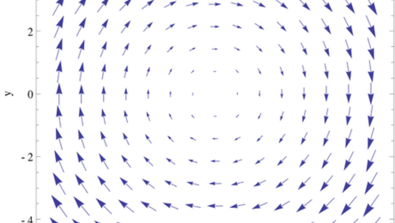
Understand what curl is. The curl, defined for vector fields, is, intuitively, the amount of circulation at any point. The operator outputs another vector field. A whirlpool in real life consists of water acting like a vector field with a nonzero curl. Above is an example of a field with negative curl (because it's rotating clockwise). The curl is recognized by curl {\displaystyle \operatorname {curl} } \operatorname {curl} or ∇ × {\displaystyle \nabla \times } \nabla \times , where the times symbol signifies the similarity of taking a cross product.

Set up the determinant. The curl of a function is similar to the cross product of two vectors, hence why the curl operator is denoted with a ∇ × . {\displaystyle \nabla \times .} \nabla \times . As before, this mnemonic only works if F {\displaystyle \mathbf {F} } {\mathbf {F}} is defined in Cartesian coordinates. ∇ × F = | x ^ y ^ z ^ ∂ / ∂ x ∂ / ∂ y ∂ / ∂ z F x F y F z | {\displaystyle \nabla \times \mathbf {F} ={\begin{vmatrix}\mathbf {\hat {x}} &\mathbf {\hat {y}} &\mathbf {\hat {z}} \\\partial /\partial x&\partial /\partial y&\partial /\partial z\\F_{x}&F_{y}&F_{z}\end{vmatrix}}} \nabla \times {\mathbf {F}}={\begin{vmatrix}{\mathbf {{\hat {x}}}}&{\mathbf {{\hat {y}}}}&{\mathbf {{\hat {z}}}}\\\partial /\partial x&\partial /\partial y&\partial /\partial z\\F_{{x}}&F_{{y}}&F_{{z}}\end{vmatrix}}

Find the determinant of the matrix. Below, we do it by cofactor expansion (expansion by minors). ∇ × F = ( ∂ F z ∂ y − ∂ F y ∂ z ) x ^ − ( ∂ F z ∂ x − ∂ F x ∂ z ) y ^ + ( ∂ F y ∂ x − ∂ F x ∂ y ) z ^ {\displaystyle \nabla \times \mathbf {F} =\left({\frac {\partial F_{z}}{\partial y}}-{\frac {\partial F_{y}}{\partial z}}\right)\mathbf {\hat {x}} -\left({\frac {\partial F_{z}}{\partial x}}-{\frac {\partial F_{x}}{\partial z}}\right)\mathbf {\hat {y}} +\left({\frac {\partial F_{y}}{\partial x}}-{\frac {\partial F_{x}}{\partial y}}\right)\mathbf {\hat {z}} } \nabla \times {\mathbf {F}}=\left({\frac {\partial F_{{z}}}{\partial y}}-{\frac {\partial F_{{y}}}{\partial z}}\right){\mathbf {{\hat {x}}}}-\left({\frac {\partial F_{{z}}}{\partial x}}-{\frac {\partial F_{{x}}}{\partial z}}\right){\mathbf {{\hat {y}}}}+\left({\frac {\partial F_{{y}}}{\partial x}}-{\frac {\partial F_{{x}}}{\partial y}}\right){\mathbf {{\hat {z}}}}

Use the formulas below as a reference. The curl does not have a simple form if F {\displaystyle \mathbf {F} } {\mathbf {F}} is in cylindrical or spherical coordinates. ( ∂ F z ∂ y − ∂ F y ∂ z ) x ^ − ( ∂ F z ∂ x − ∂ F x ∂ z ) y ^ + ( ∂ F y ∂ x − ∂ F x ∂ y ) z ^ {\displaystyle \left({\frac {\partial F_{z}}{\partial y}}-{\frac {\partial F_{y}}{\partial z}}\right)\mathbf {\hat {x}} -\left({\frac {\partial F_{z}}{\partial x}}-{\frac {\partial F_{x}}{\partial z}}\right)\mathbf {\hat {y}} +\left({\frac {\partial F_{y}}{\partial x}}-{\frac {\partial F_{x}}{\partial y}}\right)\mathbf {\hat {z}} } \left({\frac {\partial F_{{z}}}{\partial y}}-{\frac {\partial F_{{y}}}{\partial z}}\right){\mathbf {{\hat {x}}}}-\left({\frac {\partial F_{{z}}}{\partial x}}-{\frac {\partial F_{{x}}}{\partial z}}\right){\mathbf {{\hat {y}}}}+\left({\frac {\partial F_{{y}}}{\partial x}}-{\frac {\partial F_{{x}}}{\partial y}}\right){\mathbf {{\hat {z}}}} ( 1 ρ ∂ F z ∂ ϕ − ∂ F ϕ ∂ z ) ρ ^ − ( ∂ F z ∂ ρ − ∂ F ρ ∂ z ) ϕ ^ + 1 ρ ( ∂ ( ρ F ϕ ) ∂ ρ − ∂ F ρ ∂ ϕ ) z ^ {\displaystyle \left({\frac {1}{\rho }}{\frac {\partial F_{z}}{\partial \phi }}-{\frac {\partial F_{\phi }}{\partial z}}\right){\boldsymbol {\hat {\rho }}}-\left({\frac {\partial F_{z}}{\partial \rho }}-{\frac {\partial F_{\rho }}{\partial z}}\right){\boldsymbol {\hat {\phi }}}+{\frac {1}{\rho }}\left({\frac {\partial (\rho F_{\phi })}{\partial \rho }}-{\frac {\partial F_{\rho }}{\partial \phi }}\right)\mathbf {\hat {z}} } \left({\frac {1}{\rho }}{\frac {\partial F_{{z}}}{\partial \phi }}-{\frac {\partial F_{{\phi }}}{\partial z}}\right){\boldsymbol {{\hat {\rho }}}}-\left({\frac {\partial F_{{z}}}{\partial \rho }}-{\frac {\partial F_{{\rho }}}{\partial z}}\right){\boldsymbol {{\hat {\phi }}}}+{\frac {1}{\rho }}\left({\frac {\partial (\rho F_{{\phi }})}{\partial \rho }}-{\frac {\partial F_{{\rho }}}{\partial \phi }}\right){\mathbf {{\hat {z}}}} 1 r sin ⁡ θ ( ∂ ∂ θ ( F ϕ sin ⁡ θ ) − ∂ F θ ∂ ϕ ) r ^ − 1 r ( ∂ ∂ r ( r F ϕ ) − 1 sin ⁡ θ ∂ F r ∂ ϕ ) θ ^ + 1 r ( ∂ ∂ r ( r F θ ) − ∂ F r ∂ θ ) ϕ ^ {\displaystyle {\begin{aligned}{\frac {1}{r\sin \theta }}\left({\frac {\partial }{\partial \theta }}(F_{\phi }\sin \theta )-{\frac {\partial F_{\theta }}{\partial \phi }}\right)\mathbf {\hat {r}} &-{\frac {1}{r}}\left({\frac {\partial }{\partial r}}(rF_{\phi })-{\frac {1}{\sin \theta }}{\frac {\partial F_{r}}{\partial \phi }}\right){\boldsymbol {\hat {\theta }}}\\&+{\frac {1}{r}}\left({\frac {\partial }{\partial r}}(rF_{\theta })-{\frac {\partial F_{r}}{\partial \theta }}\right){\boldsymbol {\hat {\phi }}}\end{aligned}}} {\begin{aligned}{\frac {1}{r\sin \theta }}\left({\frac {\partial }{\partial \theta }}(F_{{\phi }}\sin \theta )-{\frac {\partial F_{{\theta }}}{\partial \phi }}\right){\mathbf {{\hat {r}}}}&-{\frac {1}{r}}\left({\frac {\partial }{\partial r}}(rF_{{\phi }})-{\frac {1}{\sin \theta }}{\frac {\partial F_{{r}}}{\partial \phi }}\right){\boldsymbol {{\hat {\theta }}}}\\&+{\frac {1}{r}}\left({\frac {\partial }{\partial r}}(rF_{{\theta }})-{\frac {\partial F_{{r}}}{\partial \theta }}\right){\boldsymbol {{\hat {\phi }}}}\end{aligned}}

Calculate the curl of the following function. F = ( 5 x 2 y 2 − 7 x z 3 ) x ^ + ( 4 x − 5 x y − y 4 ) y ^ + ( x z + z 2 ) z ^ {\displaystyle \mathbf {F} =(5x^{2}y^{2}-7xz^{3})\mathbf {\hat {x}} +(4x-5xy-y^{4})\mathbf {\hat {y}} +(xz+z^{2})\mathbf {\hat {z}} } {\mathbf {F}}=(5x^{{2}}y^{{2}}-7xz^{{3}}){\mathbf {{\hat {x}}}}+(4x-5xy-y^{{4}}){\mathbf {{\hat {y}}}}+(xz+z^{{2}}){\mathbf {{\hat {z}}}}

Set up the determinant. ∇ × F = | x ^ y ^ z ^ ∂ / ∂ x ∂ / ∂ y ∂ / ∂ z F x F y F z | {\displaystyle \nabla \times \mathbf {F} ={\begin{vmatrix}\mathbf {\hat {x}} &\mathbf {\hat {y}} &\mathbf {\hat {z}} \\\partial /\partial x&\partial /\partial y&\partial /\partial z\\F_{x}&F_{y}&F_{z}\end{vmatrix}}} \nabla \times {\mathbf {F}}={\begin{vmatrix}{\mathbf {{\hat {x}}}}&{\mathbf {{\hat {y}}}}&{\mathbf {{\hat {z}}}}\\\partial /\partial x&\partial /\partial y&\partial /\partial z\\F_{{x}}&F_{{y}}&F_{{z}}\end{vmatrix}} F x = 5 x 2 y 2 − 7 x z 3 {\displaystyle F_{x}=5x^{2}y^{2}-7xz^{3}} F_{{x}}=5x^{{2}}y^{{2}}-7xz^{{3}} F y = 4 x − 5 x y − y 4 {\displaystyle F_{y}=4x-5xy-y^{4}} F_{{y}}=4x-5xy-y^{{4}} F z = x z + z 2 {\displaystyle F_{z}=xz+z^{2}} F_{{z}}=xz+z^{{2}}

Calculate the determinant. ( ∂ F z ∂ y − ∂ F y ∂ z ) x ^ = 0 − 0 {\displaystyle \left({\frac {\partial F_{z}}{\partial y}}-{\frac {\partial F_{y}}{\partial z}}\right)\mathbf {\hat {x}} =0-0} \left({\frac {\partial F_{{z}}}{\partial y}}-{\frac {\partial F_{{y}}}{\partial z}}\right){\mathbf {{\hat {x}}}}=0-0 ( ∂ F z ∂ x − ∂ F x ∂ z ) y ^ = z − ( − 21 x z 2 ) {\displaystyle \left({\frac {\partial F_{z}}{\partial x}}-{\frac {\partial F_{x}}{\partial z}}\right)\mathbf {\hat {y}} =z-(-21xz^{2})} \left({\frac {\partial F_{{z}}}{\partial x}}-{\frac {\partial F_{{x}}}{\partial z}}\right){\mathbf {{\hat {y}}}}=z-(-21xz^{{2}}) ( ∂ F y ∂ x − ∂ F x ∂ y ) z ^ = ( 4 − 5 y ) − 10 x 2 y {\displaystyle \left({\frac {\partial F_{y}}{\partial x}}-{\frac {\partial F_{x}}{\partial y}}\right)\mathbf {\hat {z}} =(4-5y)-10x^{2}{y}} \left({\frac {\partial F_{{y}}}{\partial x}}-{\frac {\partial F_{{x}}}{\partial y}}\right){\mathbf {{\hat {z}}}}=(4-5y)-10x^{2}{y}

Arrive at the answer. ∇ × F = − ( z + 21 x z 2 ) y ^ + ( 4 − 5 y − 10 x 2 y ) z ^ {\displaystyle \nabla \times \mathbf {F} =-(z+21xz^{2})\mathbf {\hat {y}} +(4-5y-10x^{2}y)\mathbf {\hat {z}} } \nabla \times {\mathbf {F}}=-(z+21xz^{{2}}){\mathbf {{\hat {y}}}}+(4-5y-10x^{{2}}y){\mathbf {{\hat {z}}}} Note that we have mapped to another vector field.