Step-by-Step Guide to Removing Blank Rows in Excel (or Google Sheets)

• Highlight the blank rows in your document, right click (Windows) or Ctrl-click (Mac), and select "Delete rows" to delete blank rows manually.
• You can use the =COUNTA formula to help you find and filter blank rows so they can easily be deleted.
• Manual deletion works well for small sheets and is too time-consuming for big sheets, but the filter method works for spreadsheets of all sizes.

Using a Filter

Open your Excel document. If you have a large Excel sheet, you can use a filter to easily display all of the blank rows without having to scroll. Note that this method will work on Excel sheets with any amount of data, but is especially convenient for large and complicated sheets. This method will also work on Google Sheets, but instead of a Data tab you'll want to use the Data menu item at the top of the screen.

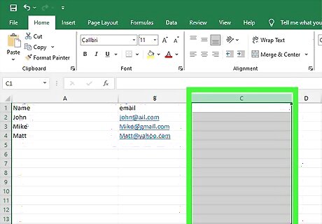
Add a new column to your document. For most sheets, it is most convenient to make this column the rightmost column, but you can also add a new column to the left of the first column if you prefer. However, you should not add the column in the middle of your data.

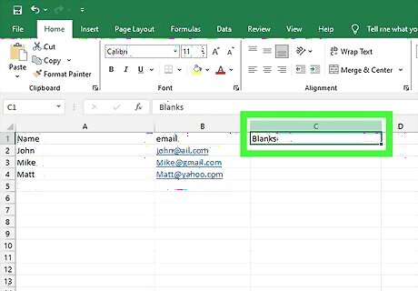
Title this column "Blanks". You don't have to worry about formatting this column as it will be deleted later.

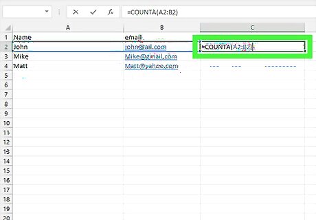
Click the cell directly under the cell that says "Blanks". In this cell enter the formula =COUNTA(XX:YY). In this formula, XX should be the first cell in the row and YY should be the last. For example, if your row starts at B2 and ends at K2, you'd write =COUNTA(B2:K2).

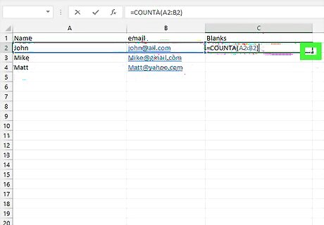
Click the dot in the lower-right corner of your formula cell and drag down. This will copy the formula to each cell and replace the row numbers in the formula with the appropriate ones for that row. Drag down to the bottom of your sheet.

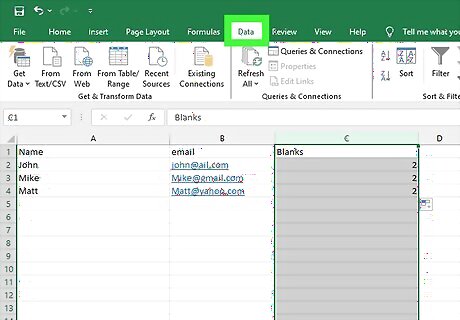
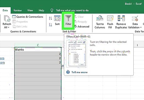
Select the cell that says "Blanks" and go to the Data tab. On Google Sheets you'll want to click the Data dropdown menu item.

Select Filter. On Google Sheets you'll want to click Create a filter. This will add filters to the headers on your sheet. If your sheet already has column filters, you can skip this step.

Click the dropdown arrow next to "Blanks". A menu will appear with various sorting options.

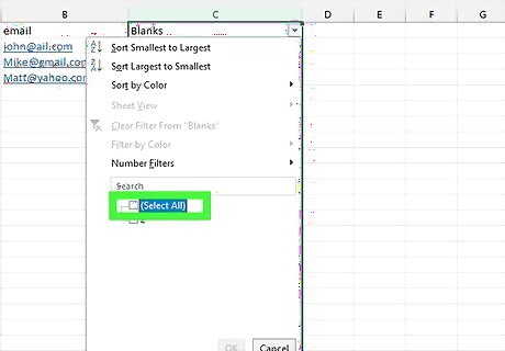
Click "Select All" to clear the checkboxes. On Google Sheets you can click the option that says "Clear" to clear all of the filter criteria.

Select "0", then click the OK button. Blank rows will have a value of "0" in the "Blanks" column, so by selecting "0", you're asking the sheet to only show you rows that fit that criteria (i.e. rows that are fully blank).

Select the blank rows. You can click the row number of the first blank row and drag down to the row number of the last blank row, or you can click the first blank row, hold down the Shift key, and click on the last blank row.

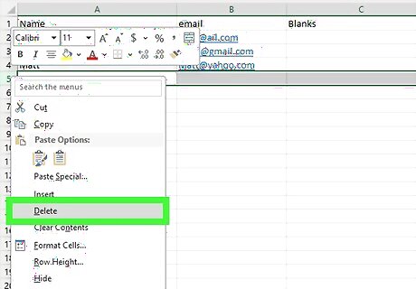
Right click any one of the selected rows and press Delete rows. On a Mac, Ctrl-click on any one of the selected rows to pull up the contextual menu, and then you can select Delete rows.

Remove the filter by pressing the Filter button again. You can do this in Google Sheets by clicking the Data dropdown and selecting Remove filter.

Click the column letter of the "Blanks" column and delete it. Simply right click the highlighted column (or Ctrl-click on Mac) and select Delete column.

Deleting Blank Rows Manually

Open your Excel document. If you have a small spreadsheet in Excel, you can manually select empty rows and delete them. If your spreadsheet is very large, you may want to consider Using a Filter. This method will also work in Google Sheets.

Click the row number next to the blank row. If you click the column number all the way on the left-hand side of the page, it will highlight the entire row. Alternatively, you can click and drag your cursor over the empty cells to select them. If you need to select multiple rows that are adjacent to one another, hold down the ⇧ Shift key and click the first and then the last row number. All of the rows in between those rows will be selected. Release the ⇧ Shift key once you're done. Alternatively, you can click and drag from the first blank row to the last blank row in a sequence to select them. If you need to select multiple rows that are not adjacent to one another, hold down the Ctrl key on Windows or the ⌘ Cmd key on Mac and click each row number. Release the Ctrl/⌘ Cmd key once you're done.

Right click any one of the selected rows and press Delete rows. On a Mac, Ctrl-click on any one of the selected rows to pull up the contextual menu, and then you can select Delete rows.